Schnakenberg System

Y. Xiao (Contributor)

L. Edelstein-Keshet: Mathematical Models in Cell Biology

Persistent Identifier

Use this permanent link to cite or share this Morpheus model:

Creating patterns using the Schnakenberg reaction-diffusion system

Introduction

We use the Schnakenberg system to generate patterns using a pair of reaction-diffusion (RD) equations, build up from 1D to 2D and explore parameter dependence.

Description

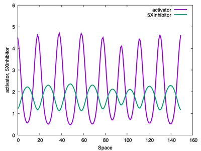
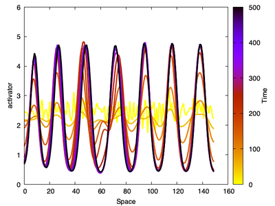
We run the Schnakenberg system of PDEs in 1D with no-flux BoundaryConditions from initial profile of noise.

Results

The final pattern (at $t = 500$) in the 1D Schnakenberg system.

A time sequence of pattern formation in the 1D Schnakenberg system, the simulation starts with random initial conditions and proceeds to form a series of peaks.

Top: a time sequence of the Schnakenberg RD system equation. Stripes are initialized, merged and sharpened due to the pattern-forming system; produced by [`Schnakenberg2Da.xml`](#downloads). Bottom: The same RD system but with random noise close to the HSS as initial conditions. A pattern of spots emerges over time, produced with [`Schnakenberg2Db.xml`](#downloads). — Top: a time sequence of the Schnakenberg RD system equation. Stripes are initialized, merged and sharpened due to the pattern-forming system; produced by `Schnakenberg2Da.xml`. Bottom: The same RD system but with random noise close to the HSS as initial conditions. A pattern of spots emerges over time, produced with `Schnakenberg2Db.xml`.

A variety of patterns formed by the Schnakenberg RD system with noisy initial conditions but with various values of the time-scale parameter $\gamma$. In each case, the system was integrated until $t = 1000$ using the Morpheus file [`Schnakenberg2Db.xml`](#downloads). — A variety of patterns formed by the Schnakenberg RD system with noisy initial conditions but with various values of the time-scale parameter $\gamma$. In each case, the system was integrated until $t = 1000$ using the Morpheus file `Schnakenberg2Db.xml`.

Simulations of the Schnakenberg system on different sized irregular domains with `noflux` `BoundaryCondition`s. Produced with Morpheus file [`Schnakenberg2Dshape.xml`](#downloads). — Simulations of the Schnakenberg system on different sized irregular domains with `noflux` `BoundaryCondition`s. Produced with Morpheus file `Schnakenberg2Dshape.xml`.

The model Schnakenberg2Dshape.xml ( | ) also requires the separate files picture1.tiff, picture2.tiff and picture3.tiff.

Model

Get this model via:

Morpheus-Link or

Download: SchnakenbergRD1D_main.xml

XML Preview

<MorpheusModel version="4">
    <Description>
        <Title>Schnakenberg RD System 1D</Title>
        <Details>Full title:		Schnakenberg System
Authors:		L. Edelstein-Keshet
Contributors:	Y. Xiao
Date:		04.06.2022
Software:		Morpheus (open-source). Download from https://morpheus.gitlab.io
Model ID:		https://identifiers.org/morpheus/M2002
File type:		Main model
Reference:		L. Edelstein-Keshet: Mathematical Models in Cell Biology
Comment:		Patterns formed by the Schnakenberg reaction-diffusion system. u is the activator and v is the inhibitor. gamma sets the time scale of the kinetics relative to the rates of diffusion. Modified from the Morpheus example Example-ActivatorInhibitor-2D (https://identifiers.org/morpheus/M0012).</Details>
    </Description>
    <Global>
        <Field symbol="u" name="activator" value="2+0.5*rand_norm(1,0.5)">
            <Diffusion rate="0.01"/>
        </Field>
        <Field symbol="v" name="inhibitor" value="1.0">
            <Diffusion rate="1"/>
        </Field>
        <Field symbol="v_5" name="5Xinhibitor" value="5">
            <Diffusion rate="0"/>
            <Annotation>v_5 is defined for plotting purposes, so that v shows up well on the plot of u.</Annotation>
        </Field>
        <System time-step="0.1" name="Schnakenberg" solver="Runge-Kutta [fixed, O(4)]">
            <Constant symbol="gamma" value="0.1"/>
            <Constant symbol="a" value="0.2"/>
            <Constant symbol="b" value="2.0"/>
            <DiffEqn symbol-ref="u">
                <Expression>gamma*(a-u+v*(u^2))</Expression>
            </DiffEqn>
            <DiffEqn symbol-ref="v">
                <Expression>gamma*(b-v*(u^2))</Expression>
            </DiffEqn>
            <Rule symbol-ref="v_5">
                <Expression>5*v</Expression>
            </Rule>
        </System>
    </Global>
    <Space>
        <Lattice class="linear">
            <Size symbol="size" value="150, 0, 0"/>
            <NodeLength value="0.2"/>
            <BoundaryConditions>
                <Condition type="noflux" boundary="x"/>
                <Condition type="noflux" boundary="-x"/>
            </BoundaryConditions>
            <Neighborhood>
                <Order>1</Order>
            </Neighborhood>
        </Lattice>
        <SpaceSymbol symbol="space"/>
    </Space>
    <Time>
        <StartTime value="0"/>
        <StopTime value="500"/>
        <SaveInterval value="0"/>
        <TimeSymbol symbol="time"/>
    </Time>
    <Analysis>
        <Logger time-step="50">
            <Input>
                <Symbol symbol-ref="u"/>
            </Input>
            <Output>
                <TextOutput file-format="csv"/>
            </Output>
            <Plots>
                <Plot time-step="50">
                    <Style line-width="3.0" style="lines"/>
                    <Terminal terminal="png"/>
                    <X-axis>
                        <Symbol symbol-ref="space.x"/>
                    </X-axis>
                    <Y-axis minimum="0" maximum="6">
                        <Symbol symbol-ref="u"/>
                        <!--    <Disabled>
        <Symbol symbol-ref="v_5"/>
    </Disabled>
-->
                    </Y-axis>
                    <!--    <Disabled>
        <Range>
            <Disabled>
                <Data/>
            </Disabled>
            <Disabled>
                <Time mode="current"/>
            </Disabled>
        </Range>
    </Disabled>
-->
                    <Color-bar reverse-palette="true">
                        <Symbol symbol-ref="time"/>
                    </Color-bar>
                </Plot>
            </Plots>
        </Logger>
        <Logger time-step="10">
            <Input>
                <Symbol symbol-ref="u"/>
            </Input>
            <Output>
                <TextOutput file-format="matrix"/>
            </Output>
            <Plots>
                <SurfacePlot time-step="10">
                    <Color-bar>
                        <Symbol symbol-ref="u"/>
                    </Color-bar>
                    <Terminal terminal="png"/>
                </SurfacePlot>
            </Plots>
        </Logger>
        <ModelGraph format="svg" reduced="false" include-tags="#untagged"/>
    </Analysis>
</MorpheusModel>

Downloads

Files associated with this model:

1D 2D BoundaryCondition Contributed Examples Domain Image Irregular Domain Noflux Partial Differential Equation PDE Reaction-diffusion System Schnakenberg System

Last updated on Tue, 25 Apr 2023